3개의 분류법을 사용하여 분류해본다.
- Rpart decision trees
- Support vector machines
- k-nearest neighbour classification
The bearings dataset
이제부터 할 분석은 4개의 베어링이 각각 7개의 상태를 가지고 있다. 이들은 서로 다른 비율로 구성된 데이터들이다.
early	failure.b2	failure.inner	failure.roller	normal	stage2	suspect
966	        37            37           608		 4344	 317	  2315
정확한 정보를 얻으려면 정확한 분류의 총 개수보다는 각 분류의 정확도 백분율을 기준으로 가중치의 정확도를 계산해야 한다. 또한 데이터 세트에서 무작위로 선택하지 않고 클래스에서 동등한 비율로 가지고 와야한다.
Technique 1: Rpart Decision Trees
decision tree는 features에 대해 질문의 흐름을 담고있는 플로우차트와 같다. 스무고개와 같이 깊어질수록 구체적으로 질문하고 분류에 대한 정보를 제공한다. 트리를 만드는 프로세스를 rule induction이라고 하며 rule은 데이터의 학습 세트에서 직접 만들어진다. 의사결정트리는 일반적으로 이진트리이며 데이터를 두 세트로 분할한다.
먼저 Rpart tree를 작성해보자.
library("rpart")
# Calculate accuracy weighted by counts per class
weighted.acc <- function(predictions, actual)
{
freqs <- as.data.frame(table(actual))
tmp <- t(mapply(function (p, a) { c(a, p==a) }, predictions, actual, USE.NAMES=FALSE)) # map over both together
tab <- as.data.frame(table(tmp[,1], tmp[,2])[,2]) # gives rows of [F,T] counts, where each row is a state
acc.pc <- tab[,1]/freqs[,2]
return(sum(acc.pc)/length(acc.pc))
}
# Read in the relabelled best features
basedir <- "/Users/vic/Projects/bearings/bearing_IMS/1st_test/"
data <- read.table(file=paste0(basedir, "../all_bearings_relabelled.csv"), sep=",", header=TRUE)
# Read in training set row numbers
train <- read.table(file=paste0(basedir, "../train.rows.csv"), sep=",")[,1]
# Set up class weights to penalise the minority classes more
cw1 <- rep(1, 7) # all equal
cw2 <- c(10, 100, 100, 10, 1, 10, 1) # 1/order of count
freqs <- as.data.frame(table(data$State))
cw3 <- cbind(freqs[1], apply(freqs, 1, function(s) { length(data[,1])/as.integer(s[2])})) # 1/weight
class.weights <- rbind(cw1, cw2, cw3[,2])
colnames(class.weights) <- c("early", "failure.b2", "failure.inner", "failure.roller", "normal", "stage2", "suspect")
results <- matrix(ncol=4, nrow=0)
models <- list()
for (c in 1:length(class.weights[,1]))
{
data.weights <- do.call(rbind, Map(function(s)
{
class.weights[c,s]
}, data$State))
cat("Run for c", c, "\n")
model <- rpart(State ~ ., data=data[train,-1], weights=data.weights[train], method="class")
pred <- predict(model, data[,-1], type="class")
tacc <- weighted.acc(pred[train], data[train,2])
wacc <- weighted.acc(pred[-train], data[-train,2])
pacc <- sum(pred[-train]==data[-train,2])/length(pred[-train])
results <- rbind(results, c(tacc, wacc, pacc, c))
models[[(length(models)+1)]] <- model
}
# Visualise the best tree
best.row <- match(max(results[,2]), results[,2])
best.rpart <- models[[best.row]]
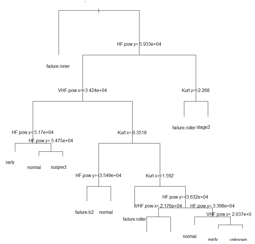
plot(best.rpart, compress=TRUE)
text(best.rpart)
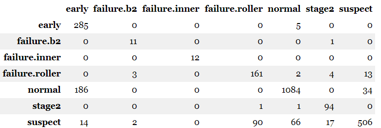
# And the confusion matrix
pred <- predict(best.rpart, data[,-1], type="class")
table(data[-train,2], pred[-train])
# Save everything
save(results, file=paste0(basedir, "../../models/rpart.results.obj"))
save(models, file=paste0(basedir, "../../models/rpart.models.obj"))
write.table(results, file=paste0(basedir, "../../models/rpart.results.csv"), sep=",")
save(best.rpart, file=paste0(basedir, "../../models/best.rpart.obj"))3가지 weightings로 테스트해보았다.
- cw1 : all classes equally weighted
- cw2 : classes weighted by order using powers of 10;
- cw3 : classes weighted by 1/count of samples in the dataset
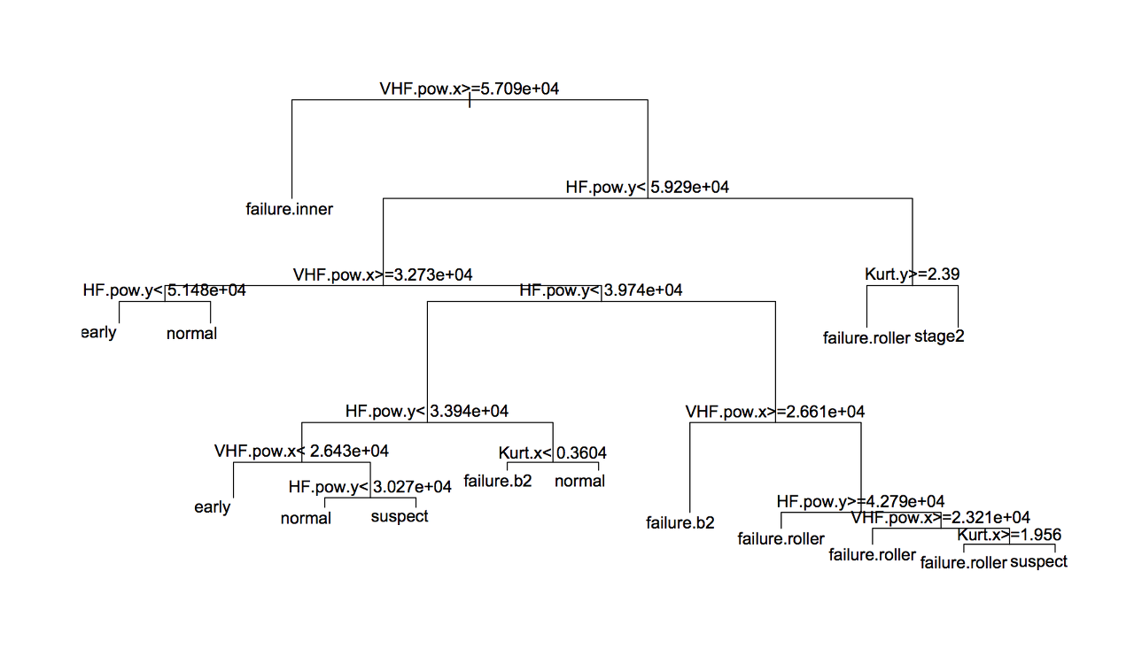
여기서 가장 좋았던 트리는 cw2로 90.3%의 정확도를 보였다. cw2는 다음과 같이 생겼다.
confusion matrix는 다음과 같다.
Technique 2 : Support Vector Machines
classification는 두 개의 클래스를 나누는 명확한 경계선을 그리기 어렵다. 일반적으로 클래스에 속하는 점들은 약간의 중첩이 존재하며 보통 잘못 분류된 점들이다. feature design의 생각은 클래스들간의 거리가 가장 먼 파라미터를 찾아내는 것이다. 그리고 경계선의 점들이 적어야 한다.
Support Vector Machines은 이런 문제점에 대해 데이터의 차원을 높여 해결한다. 피처 공간에서 클러스터간에 겹치는 부분이 있따면 더 높은 차원의 공간에 그것들을 구분지을 수 있는 선을 그을 수 있기 때문이다. 차원은 kernel function을 통해 증가하고 주로 Radial Basis Function이 선택된다.
R에서 SVM은 e1071이라는 라이브러리를 사용한다. 코드는 다음과 같다.
library("e1071")
# Calculate accuracy weighted by counts per class
weighted.acc <- function(predictions, actual)
{
freqs <- as.data.frame(table(actual))
tmp <- t(mapply(function (p, a) { c(a, p==a) }, predictions, actual, USE.NAMES=FALSE)) # map over both together
tab <- as.data.frame(table(tmp[,1], tmp[,2])[,2]) # gives rows of [F,T] counts, where each row is a state
acc.pc <- tab[,1]/freqs[,2]
return(sum(acc.pc)/length(acc.pc))
}
# Read in the relabelled best features
basedir <- "/Users/vic/Projects/bearings/bearing_IMS/1st_test/"
data <- read.table(file=paste0(basedir, "../all_bearings_relabelled.csv"), sep=",", header=TRUE)
# Read in training set row numbers
train <- read.table(file=paste0(basedir, "../train.rows.csv"), sep=",")[,1]
# Set up class weights to penalise the minority classes more
cw1 <- rep(1, 7) # all equal
cw2 <- c(10, 100, 100, 10, 1, 10, 1) # 1/order of count
freqs <- as.data.frame(table(data$State))
cw3 <- cbind(freqs[1], apply(freqs, 1, function(s) { length(data[,1])/as.integer(s[2])})) # 1/weight
cw4 <- c(10, 1, 1, 10, 100, 10, 100) # order of count
class.weights <- rbind(cw1, cw2, cw3[,2], cw4)
colnames(class.weights) <- c("early", "failure.b2", "failure.inner", "failure.roller", "normal", "stage2", "suspect")
results <- matrix(ncol=5, nrow=0)
models <- list()
for (c in 1:length(class.weights[,1]))
{
for (g in seq(-6, -1, by = 1))
{
for (cost in 0:3)
{
cat("Run for weights", c, ", g", 10^g, "and c", 10^cost, "\n")
# Data are scaled internally in svm, so no need to normalise
model <- svm(State ~ ., data=data[train,-1], class.weights=class.weights[c,], gamma=10^g, cost=10^cost)
pred <- predict(model, data[,-1], type="class")
wacc <- weighted.acc(pred[-train], data[-train,2])
pacc <- sum(pred[-train]==data[-train,2])/length(pred[-train])
results <- rbind(results, c(10^g, 10^cost, c, wacc, pacc))
models[[(length(models)+1)]] <- model
}
}
}
# Save for now
save(results, file=paste0(basedir, "../../models/svm.results.obj"))
save(models, file=paste0(basedir, "../../models/svm.models.obj"))
write.table(results, file=paste0(basedir, "../../models/svm.results.csv"), sep=",")
best.row <- match(max(results[,4]), results[,4])
best.svm <- models[[best.row]]
save(best.svm, file=paste0(basedir, "../../models/best.svm.obj"))
# Visualise
library("RColorBrewer")
pal <- brewer.pal(10, "RdYlGn")
cols <- do.call(rbind, Map(function(a)
{
if (a>0.88) pal[1]
else if (a > 0.86) pal[2]
else if (a > 0.84) pal[3]
else if (a > 0.82) pal[4]
else if (a > 0.8) pal[5]
else if (a > 0.7) pal[6]
else if (a > 0.6) pal[7]
else if (a > 0.5) pal[8]
else if (a > 0.3) pal[9]
else pal[10]
}, results[,4]))
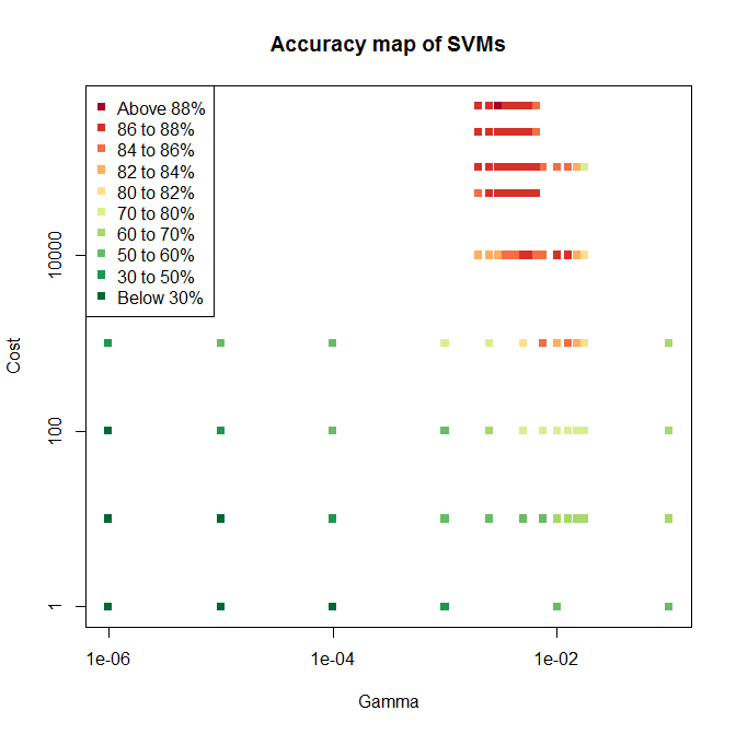
plot(results[,2] ~ results[,1], log="xy", col=cols, pch=15, xlab="Gamma", ylab="Cost", main="Accuracy map of SVMs")
labs <- c("Above 88%", "86 to 88%", "84 to 86%", "82 to 84%", "80 to 82%", "70 to 80%", "60 to 70%", "50 to 60%", "30 to 50%", "Below 30%")
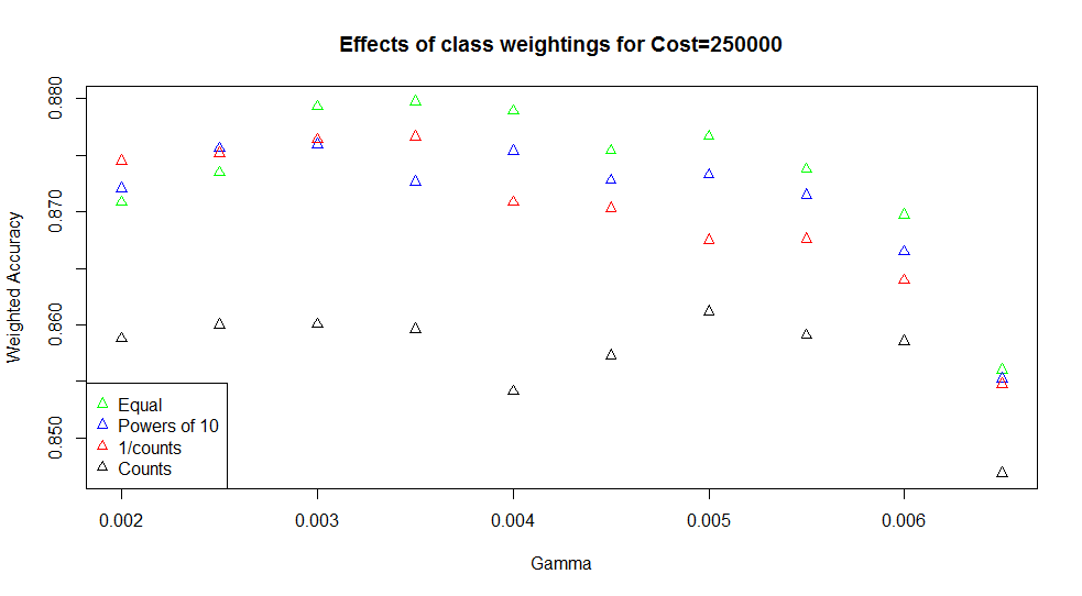
legend("topleft", labs, col=pal, pch=15)RBF kernel을 사용하기 위해 2개의 파라미터를 사용한다. 하나는 misclassifications의 cost인 C이고 하나는 RBF의 파라미터인 γ이다. grid search를 통해 적합한 값을 찾으며 svm은 모든 조합을 학습한다. 정확도를 비교하면 좋은 조합을 찾을 수 있으며 세분화하여 두 번째 그리드 검색을 설정한다. 모든 검색을 끝내면 다음과 같은 그래프가 나온다.
나는 안해봤지만 원작자는 다른 파라미터를 사용해봤다고 한다. 그 중 cw1이 가장 best했다.
'미분류 > R' 카테고리의 다른 글
| Understanding data science: classification with neural networks in R (0) | 2019.06.12 |
|---|---|
| Understanding data science: clustering with k-means in R (0) | 2019.06.11 |
| R 기본 (추가 중) (0) | 2019.06.05 |
| Understanding data science: dimensionality reduction with R (0) | 2019.06.04 |
| Understanding data science:designing useful features with R (0) | 2019.06.03 |


